Final project 3.1 Final Project
3.1 - Network Analysis of the Human Protein-Protein Interactome
Table of Contents
Introduction:
Project Summary
Human protein-protein interaction (PPI) networks provide valuable insight into the functionality of proteins beyond what is detailed in the human proteome.
In this project, we hope to visualize the structure of the human PPI network - which was obtained from two different databases - as well as determine the distribution of the degree and betweenness centrality measurements for the proteins within said network, using both our own proposed tool as well as the bioinformatics software Cytoscape. Furthermore, we would like to characterize any statistically significant differences between the proteins containing and not containing SNPs in Carl’s genome. Finally, we also perform a hierarchical analysis of the PPI network.
For project 3.1, protein-protein interaction (PPI) data were downloaded from two different databases: The Database of Interacting Proteins (DIP) and the Molecular Interaction Database (MINT). We filtered the edges where one or two of the proteins did not have the UniProtID, which constituted less than 5% of the total proteins of interest. The former database generated 4904 distinct proteins with 7,387 interactions, while the latter yielded 4584 distinct proteins with 12,655 interactions.
Coding:
Documentation:
Summary:
Hussein coded a Python program that calculates the betweenness centrality and degree centrality measurements for each node in the PPI network. Figures 3-6 show the distributions for the degree and betweenness centralities outputted by Hussein’s program. The observations of these distributions will be discussed in the following section.
Separating SNP-Containing Proteins from Non-SNP-Containing Proteins
To help separate the proteins that contain SNPs in Carl’s genome from those that do not, the proteins’ UniProt IDs were used; that is, the proteins from the data file Carl_Coding_SNP_Map.csv – obtained from Carl’s Game of Genomes blog – were mapped to the proteins from the database using the corresponding UniProtKB ID-ENSEMBL Transcript ID pairs. The total number of SNP-containing proteins is 375 in the DIP database and 306 in the MINT database.
Calculation of Degree Centrality and Betweenness Centrality
Centrality Measure Definitions
Next, the degree centrality and betweenness centrality measurements were calculated for each node. It is first important to define these two measures. The former is equivalent to the number of the links a node has. On the other hand, the betweenness centrality is defined as the number of times a node is located on the shortest path between two other nodes. In mathematical terms, the two measures are defined as follows: For a graph $G := (V, E)$ and given a node $n$: where $\sigma_{lm}$ is the total number of shortest paths between distinct nodes $l$ and $m$.
Given an input CSV file with three columns corresponding to protein interactor A, protein interactor B, and weights (for an example, see sample_processed.csv), Hussein’s code computes the degree centrality and betweenness centrality for each node within the network. The specific documentation for each line of the code from Hussein can found below:
Script Coding_3_1.py is rife with self-explanatory comments.
Required Packages:
matplotlib and numpy
Inputs:
- A file that with the edges in the PPI network: with IDs of connected proteins in the first two columns (submitted sample_processed.csv is a selected sample from DIP network with 1000 edges and 1199 nodes/proteins)
- A file with list of protein IDs that include SNPs (submitted Carl_Coding_SNP_Map.csv is a sample file). For Carl’s SNP proteins, they were identified as per per ENSEMBLE IDs in coding SNPs file and mapped to their UniProt IDs.
- Default is unweighted PPI networks. Accordingly, third column is optional: if not empty, it should include the weight of the edge so that the script accommodates weighted graphs.
Output:
Degree centrality and betweenness centrality distributions plotted for proteins with and without SNPs.
Results:
The output of Hussein’s code can be found in the coding folder of Github. The specific graphical outputs of his program are visualized in Figures 3-6. A comparison of his code with the output of Cytoscape can be found in the following pipeline section.
Pipeline:
Documentation:
Summary
For the pipeline portion of the project, Dingjue ran analyses in Cytoscape and plotted the resulting distributions for centralities in R using the ggplot2 package. The outputs from Dingjue’s code can be found in Figures 7-10. Furthermore, Dingjue conducted a hierarchical analyses of the PPI network, the results of which can be found in this report.
Visualizing the PPI Network
The interactions between different proteins can be best represented by an undirected graph, where the individual proteins are represented by nodes and their mutual interactions are represented by links. The corresponding graphs generated from the protein-protein interactions cataloged in the DIP and MINT database were created by the bioinformatics software platform Cytoscape (see Figures 1 and 2, respectively). Green nodes represent proteins that do not contain SNPs in Carl’s genome, whereas red ones represent proteins that do. Links are characterized by blue edges. Moreover, node size is directly proportional to the degree of said node; namely, bigger nodes have more links and are thus more likely to be characterized as “hubs”. Finally, different network motifs are summarized at the bottom of png images.
Results:
Comparison of Centrality Measurement Calculations from the Proposed Tool
To confirm that the proposed tool is a good calculator of the centrality measurements of interest, we compare the specific values generated by Hussein’s code to those found by the Cytoscape program. We looked at the top 10 proteins with the highest betweenness centrality and degree centrality values within the MINT and DIP databases and compared those values generated by Hussein’s code to those by Cytoscape (indicated in the tables by “Coding” and “Cytoscape”, respectively in Tables 1-4 found in the Table Appendix).
Overall, the protein names and degree centrality values for these proteins remain relatively stable between the two programs. In our first run through, however, we noted that there were differences in the betweenness centrality calculation; specifically, the top 10 proteins from the Cytoscape software all had betweenness centrality values of 1.0. This value does not make sense as it would suggest that these nodes are included in all the shortest paths for all the node pairs (l,m). Further exploration into this issue suggested that this output of 1.0 is due to a systematic error in Cytoscape.
Running the Cytoscape software again with updates in the program resulted in the histograms and the tables shown in the appendix. Notice that there are no nodes with betweenness centrality of 1.0. Furthermore, from a qualitative standpoint, by comparing the outputs of the graphs made by Hussein’s code (Figures 3-6) and Dingjue’s program (Figures 7-10), it becomes evident that the distributions are quite similar.
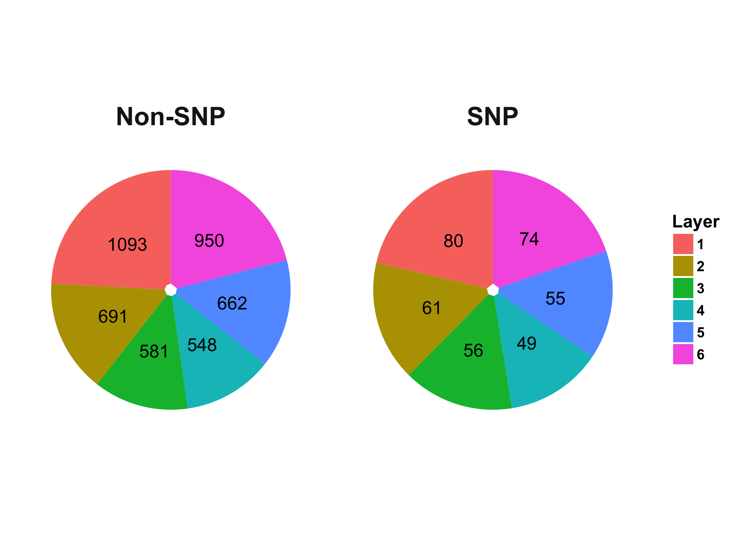
PPI Network Hierarchical Analysis
We note that the PPI networks generated from the DIP and MINT databases are undirected. However, hierarchical analyses work best on directed networks.
It was hard to find available online tools or algorithms to use that could conduct hierarchical analyses of undirected graphs. For this section, Dingjue implemented an algorithm created by Cheng et al. called HirNet (originally used to determine the hierarchical structure of the phosphorylome and regulome). This algorithm resolves the hierarchical network structure and calculates the hierarchy score for directed networks. Here, HirNet is used only to catch a glimpse of the network structure; it does not necessarily reflect regulatory features of the PPI network.
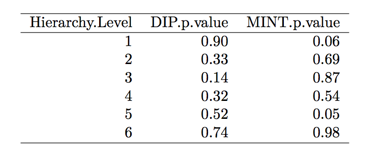
The DIP and MINT network have been cut into six layers. Fisher’s exact test was used to test the enrichment of proteins with SNP in Carl’s genome in different layers. The distribution of proteins in the six hierarchical layers is visualized below in the pie graphs.
Distribution of Proteins in the Hierarchical Layers of PPI Network Generated from DIP Database:
Distribution of Proteins in the Hierarchical Layers of PPI Network Generated from MINT Database:
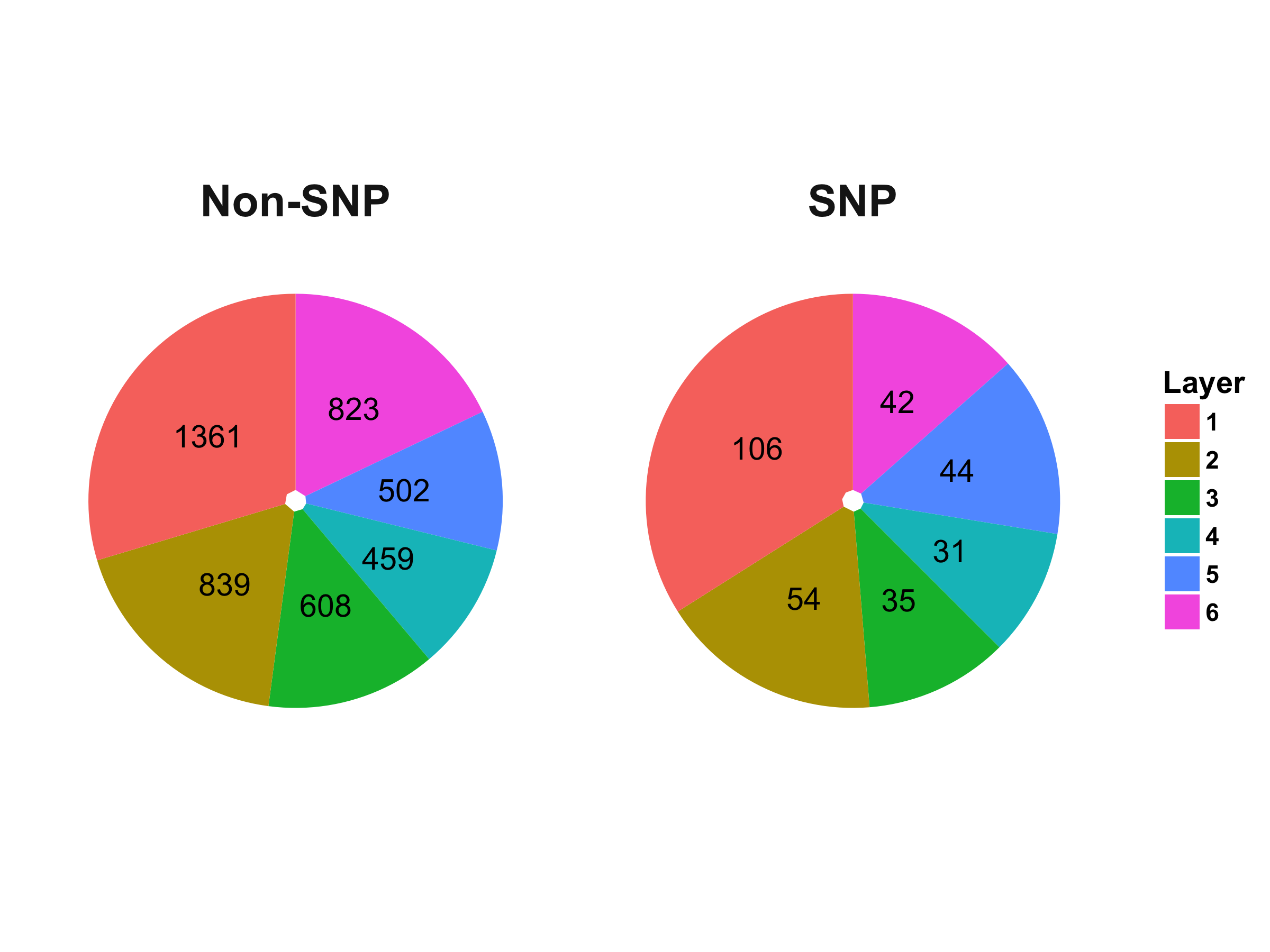
Based on the result of Fisher’s exact test ($\alpha$ = 0.05), there is no significant enrichment in any layers for the PPI network, which may indicate that proteins with SNPs are not clustered or scattered in any statistically significant patterns compared to those without SNPs.
Writing:
Observations on Centrality Measurements
This section constitutes the writing assignment proposed by the Project 3.1 guidelines. For the following sections, please refer to Figures 3 through 10.
Degree Centrality
From Barabasi and Oltvai’s review on network biology, we know that random networks tend to follow a Poisson distribution and scale-free networks tend to follow a power law (2004). For both the DIP and MINT databases, we see that the distribution of degree centrality follows a power law distribution rather than a Poisson distribution, evidenced by a large number of nodes with few links and a small number of nodes with a lot of classified as the hubs).
With regards to the SNPs vs. non-SNP proteins, it appears that there is a higher percentage of proteins with fewer links in non-SNP proteins as compared to SNP proteins.
Note: we notice that there are no counts nodes with a degree greater than 50 (as a conservative estimate). This suggests that there may be no central protein that interacts with more than 50 other proteins.
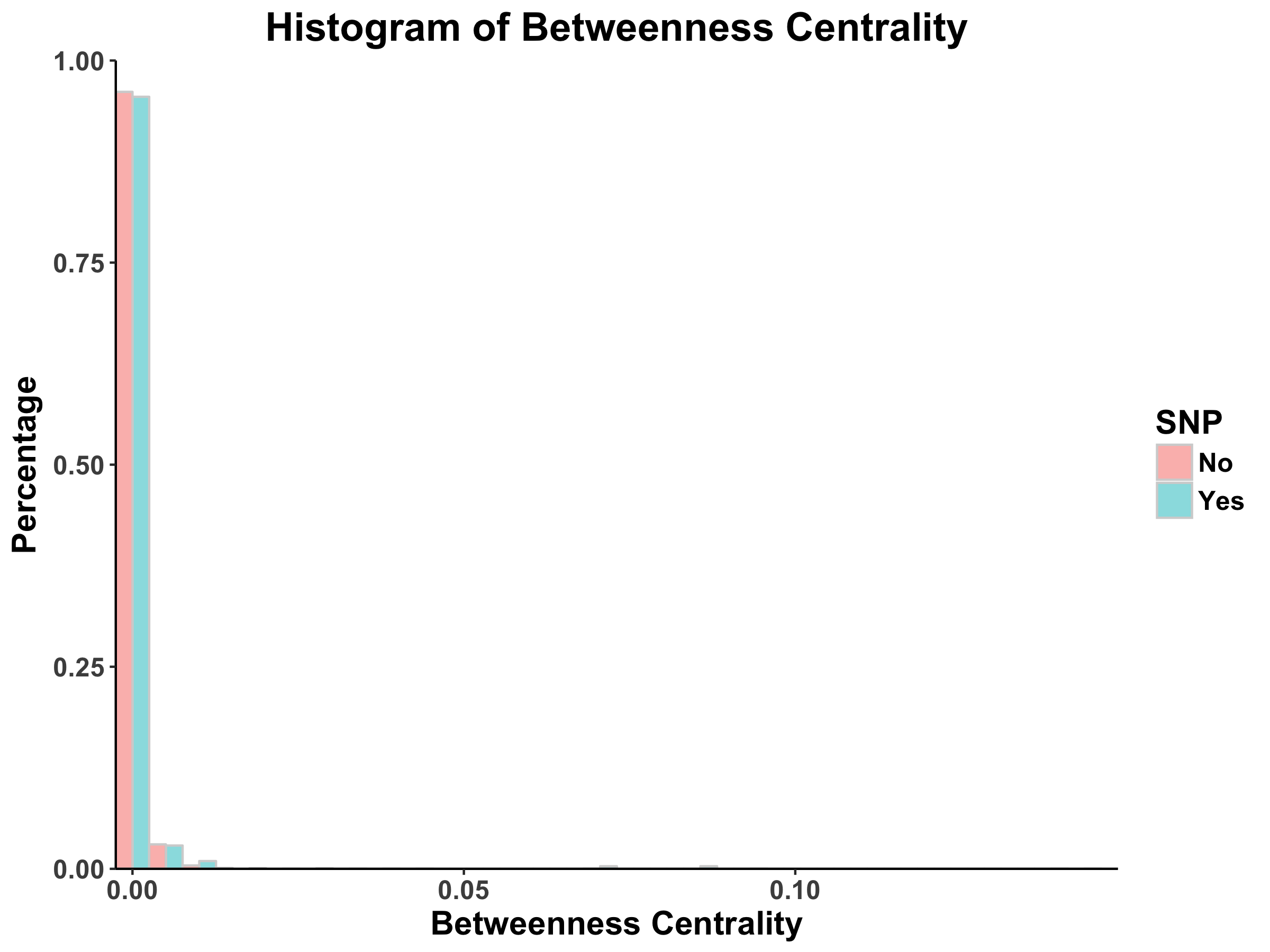
Betweenness Centrality
Looking at the histograms of betweenness centrality, we again see that these distributions follow the power law. This finding means that there are many nodes/proteins that are closely connected.
Comparing the SNP-containing vs. non-SNP-containing proteins, we see that the betweenness centrality is more distributed in the former as compared to the latter. That is, there are more proteins with higher betweenness centrality in the SNP-containing proteins. For example, there are more SNP-containing proteins that have higher betweenness centrality (between 0.50 and 1.0) than those without, suggesting that removing SNP-containing proteins has a higher probability of disrupting the PPI network. This finding is interesting, as it implies that proteins with more centrality tend to harbor more SNPs. However, there may be potential confounding variables, such as protein size and binding site accessibility, which may require further investigation. Moreover, we have to determine whether these differences between distributions are actually statistically significant…
Permutation Tests for Degree and Betweenness Centrality
Permutation tests can determine whether there are statistically significant differences in the distributions of centrality measures for proteins with SNP and no SNPs.
In these tests, we randomly label proteins as either having SNPs or no SNPs and compare the distributions of the means. Dingjue ran the permutation tests and found no statistically significant difference between the proteins containing Carl’s SNPs and those not containing his SNPs at a significance level of $\alpha = 0.05$. Therefore, while it may seem that there are local differences in the distribution of SNP vs. non-SNP-containing proteins, there is actually no statistically significant difference among the distributions.
Why Are These Observations Important?
Why are we interested in studying the distribution of degree and betweenness centrality?
According to Barabasi and Oltvai, the degree of connectedness of a protein - quantified by both the degree and betweenness centrality measures - has an important role in determining the importance of a protein within a network, i.e. would the deletion of the node have a significant impact on the network structure?
In a scale-free network - such as the human PPI network - a majority of the nodes do not have a major effect on the network’s integrity since they (1) do not have many links (low degree centrality) and (2) are not in the “middle” of other protein interactors (low betweenness centrality). As a result, a majority of the proteins are not essential for the network
At the same time, studying those nodes with high measures of centrality can lead to the discovery of important human proteins, the removal of which can be detrimental to the system. That is, a higher centrality measurement indicates a more deleterious mutation phenotype. Using the proposed tool to compute a protein’s betweenness and degree centralities within the PPI network can, therefore, allow for a rudimentary understanding of the mutation phenotype of said protein.
As expected, we do not observe SNP-containing proteins among the ten proteins with the highest measures of centrality (see Tables 1-4). These proteins are among the more important “nodes” within this network, and so we would expect less variability within them (therefore, less chance of having variants, such as SNPs).
On a network-wide scale, these centrality measures are important to determine the relative distributions and connectedness of the proteins within the PPI network.
Conclusions:
In this project, a tool to calculate the degree centrality and betweenness centrality of nodes within the PPI network was proposed. Since (1) from a qualitative viewpoint, the graphs for the centrality measures generated by both Hussein’s code and Cytospace look similar and (2) from a quantitative viewpoint, the values for the computed betweenness and degree centrality values for the “top 10” proteins are relatively close between the two software, we can propose Hussein’s code as a tool for calculating the degree centrality and betweenness centrality of proteins. Furthermore, in our analysis, we did not find statistically significant differences between the centrality measure distributions of proteins containing and not containing SNPs. With regards to the hierarchical analysis of the PPI network, there also does not seem to be any statistically significant patterns for protein distribution among different hierarchical layers.
Source code
References:
Barabasi, A.L. and Oltvai, Z.N., 2004. Network biology: understanding the cell’s functional organization. Nature reviews genetics, 5(2), pp.101-113.
Gerstein, M.B., Kundaje, A., Hariharan, M., Landt, S.G., Yan, K.K., Cheng, C., Mu, X.J., Khurana, E., Rozowsky, J., Alexander, R. and Min, R., 2012. Architecture of the human regulatory network derived from ENCODE data. Nature, 489(7414), pp.91-100.
Shannon, P., Markiel, A., Ozier, O., Baliga, N.S., Wang, J.T., Ramage, D., Amin, N., Schwikowski, B. and Ideker, T., 2003. Cytoscape: a software environment for integrated models of biomolecular interaction networks. Genome research, 13(11), pp.2498-2504.
Appendix:
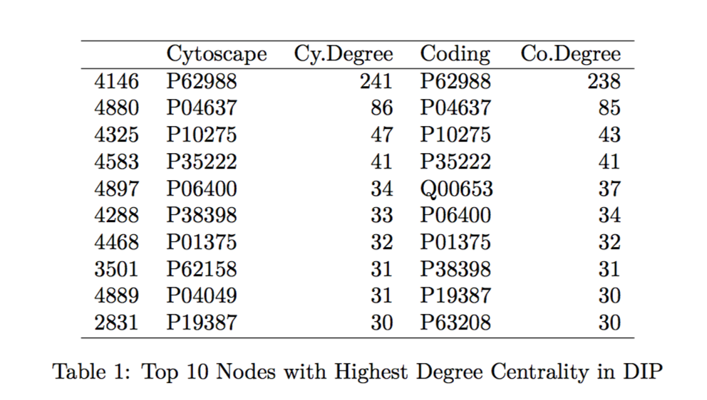
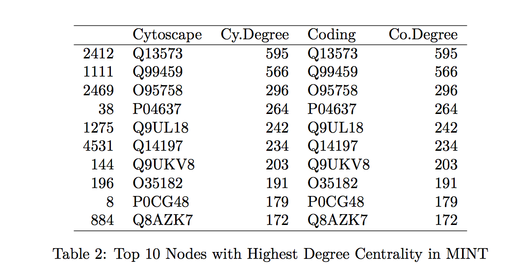
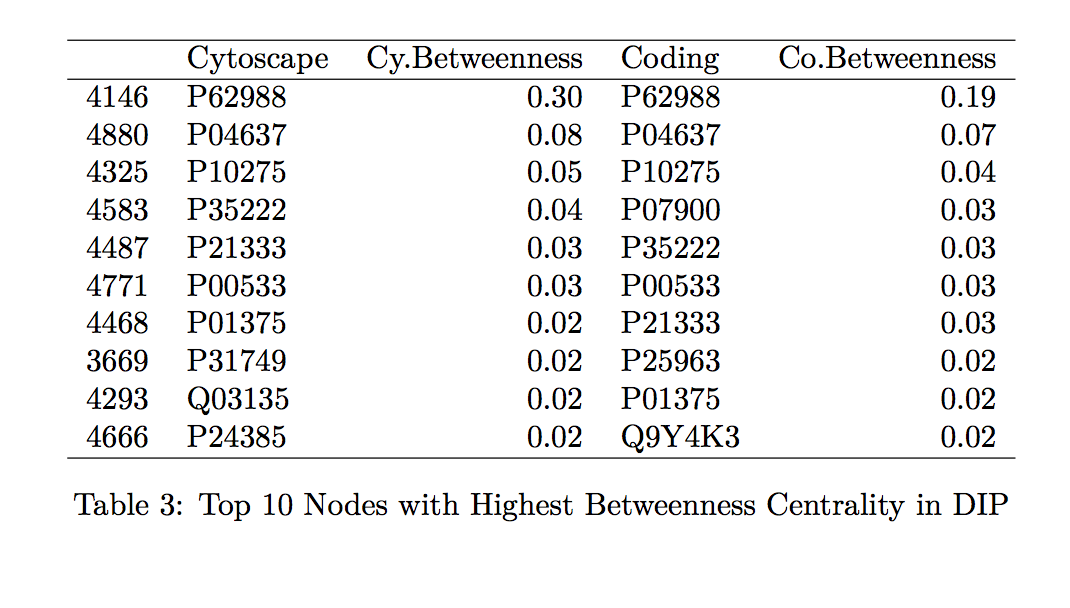
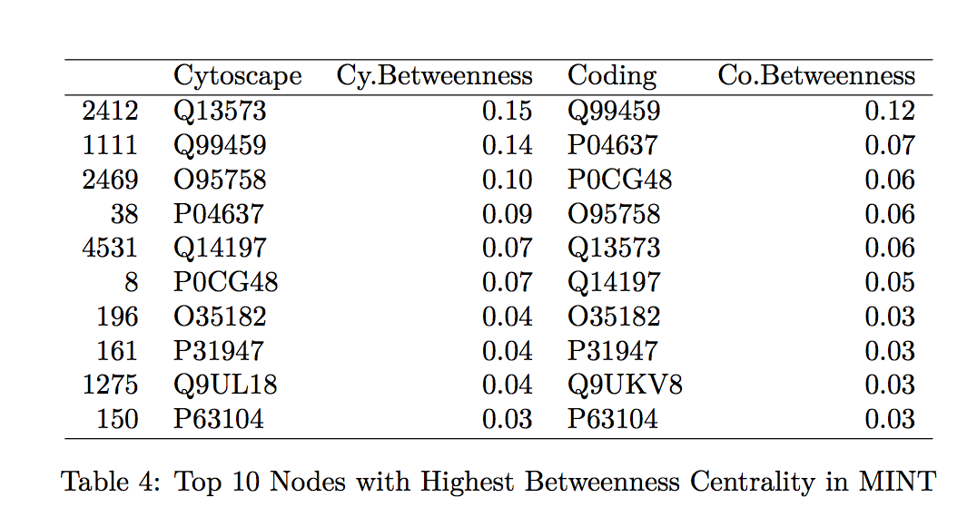
Figure 1: PPI Network Generated from DIP Database
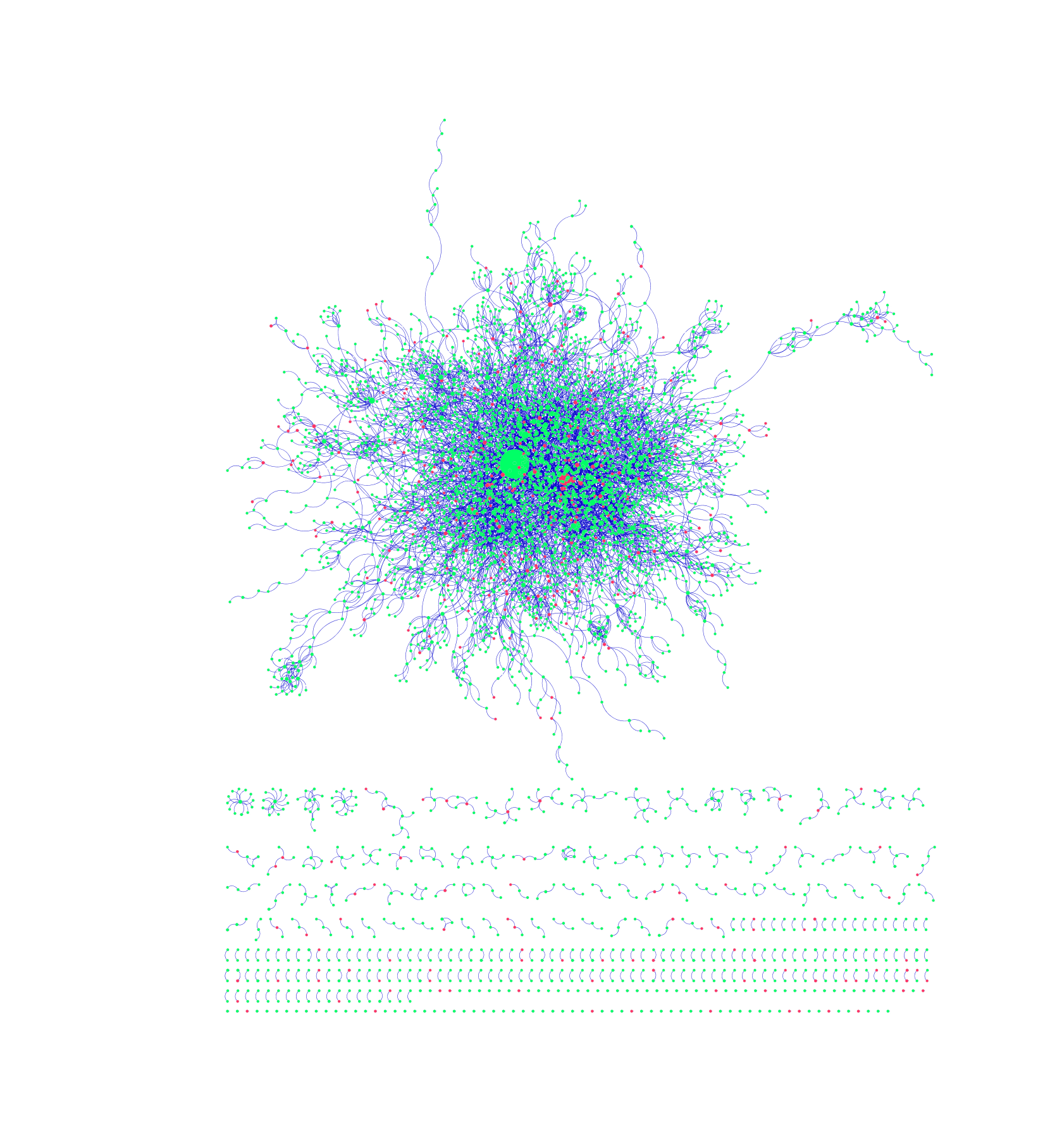
Figure 2: PPI Network Generated from MINT Database
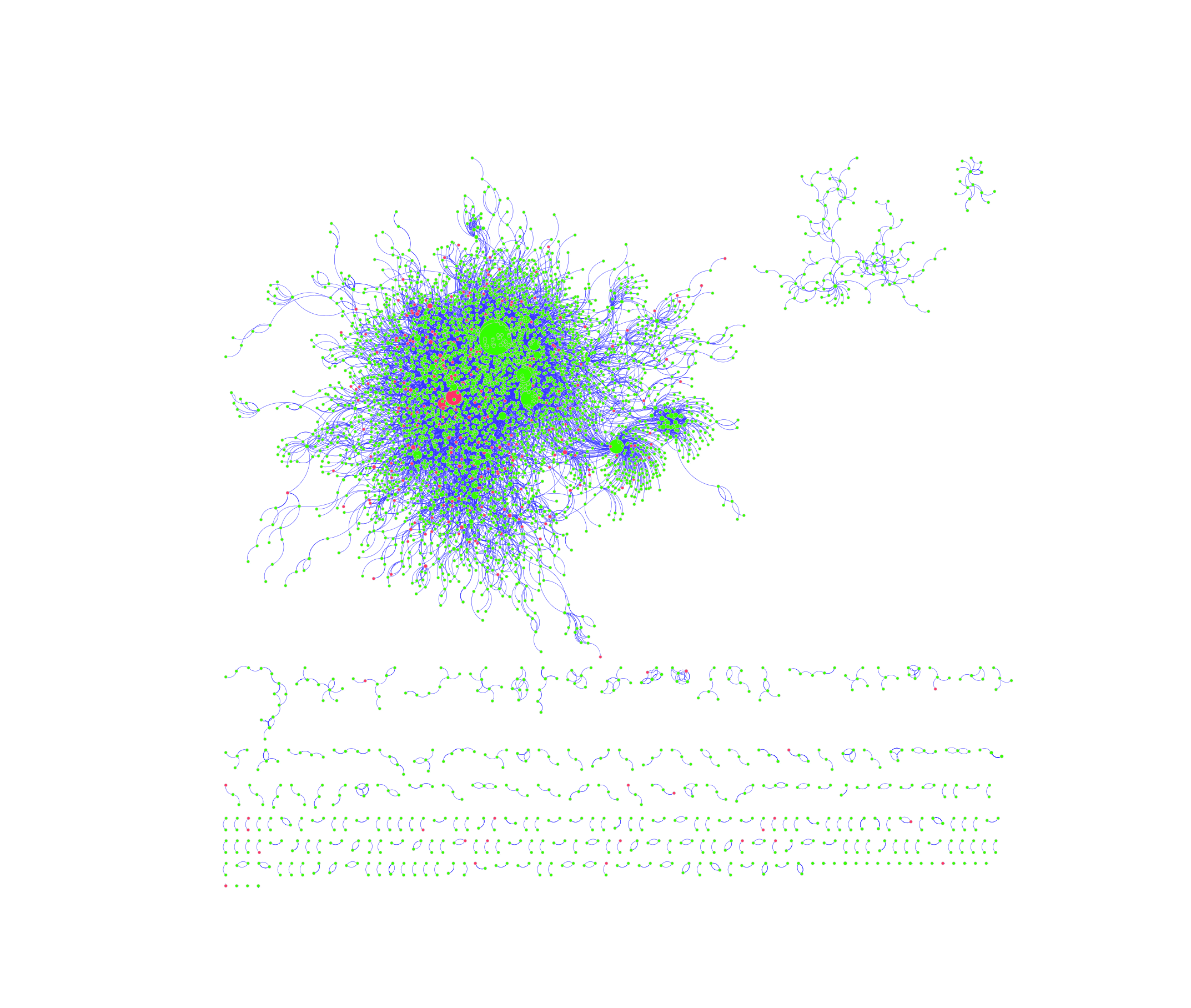
Figure 3: Degree Centrality Distribution in DIP Database Calculated by Hussein’s Code
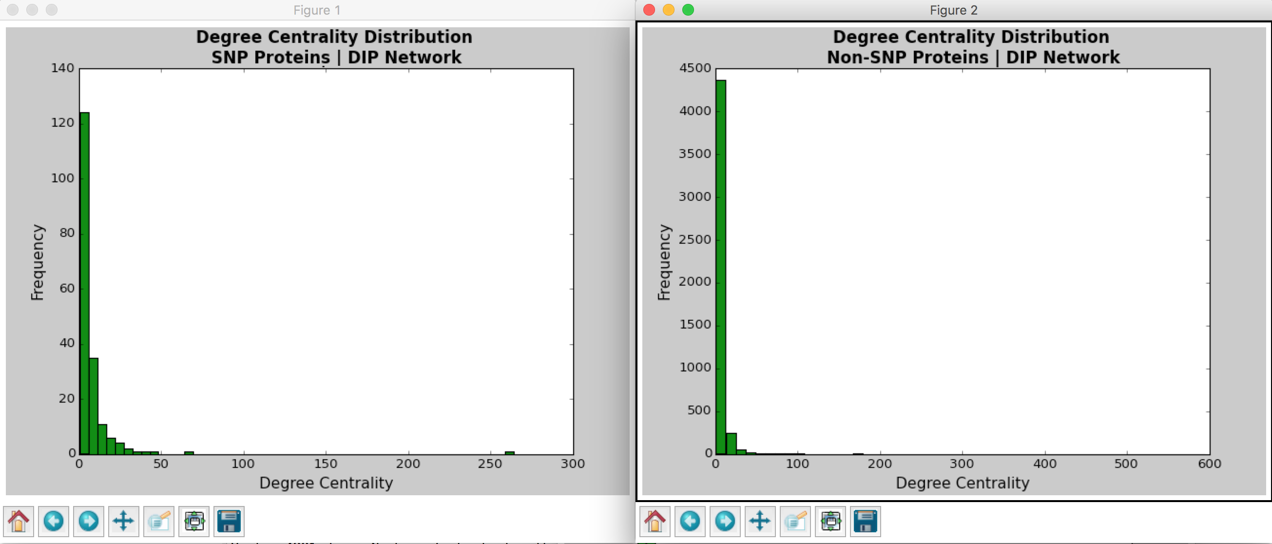
Figure 4: Betweenness Centrality Distribution in DIP Database Calculated by Hussein’s Code
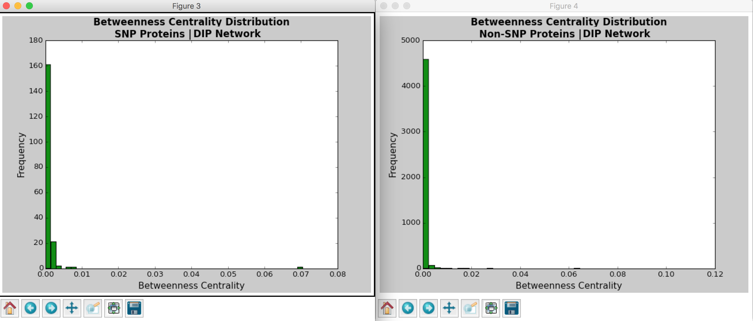
Figure 5: Degree Centrality Distribution in MINT Database Calculated by Hussein’s Code
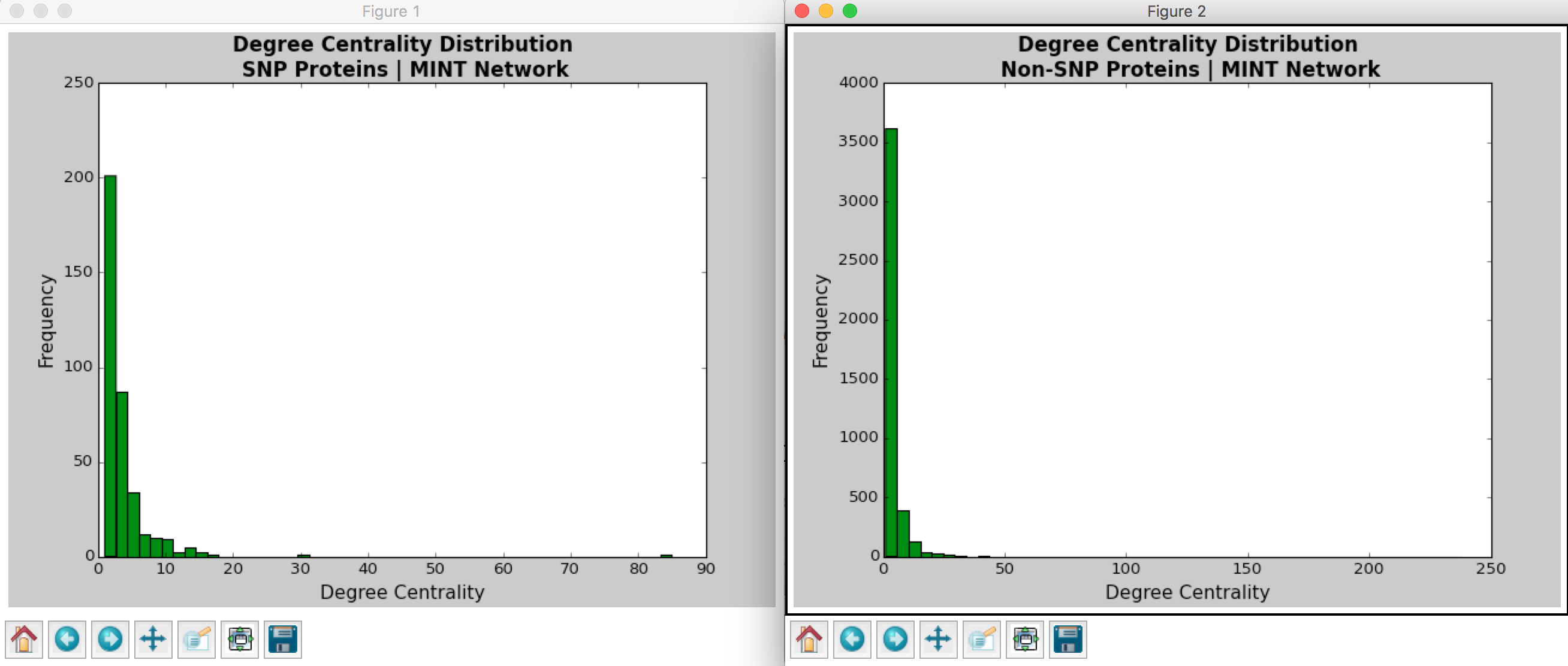
Figure 6: Betweenness Centrality Distribution in MINT Database Calculated by Hussein’s Code
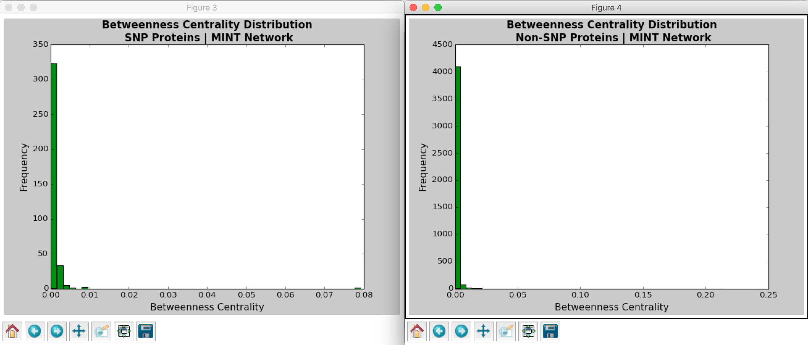
Figure 7: Degree Centrality Distribution in DIP Database Calculated by Cytoscape
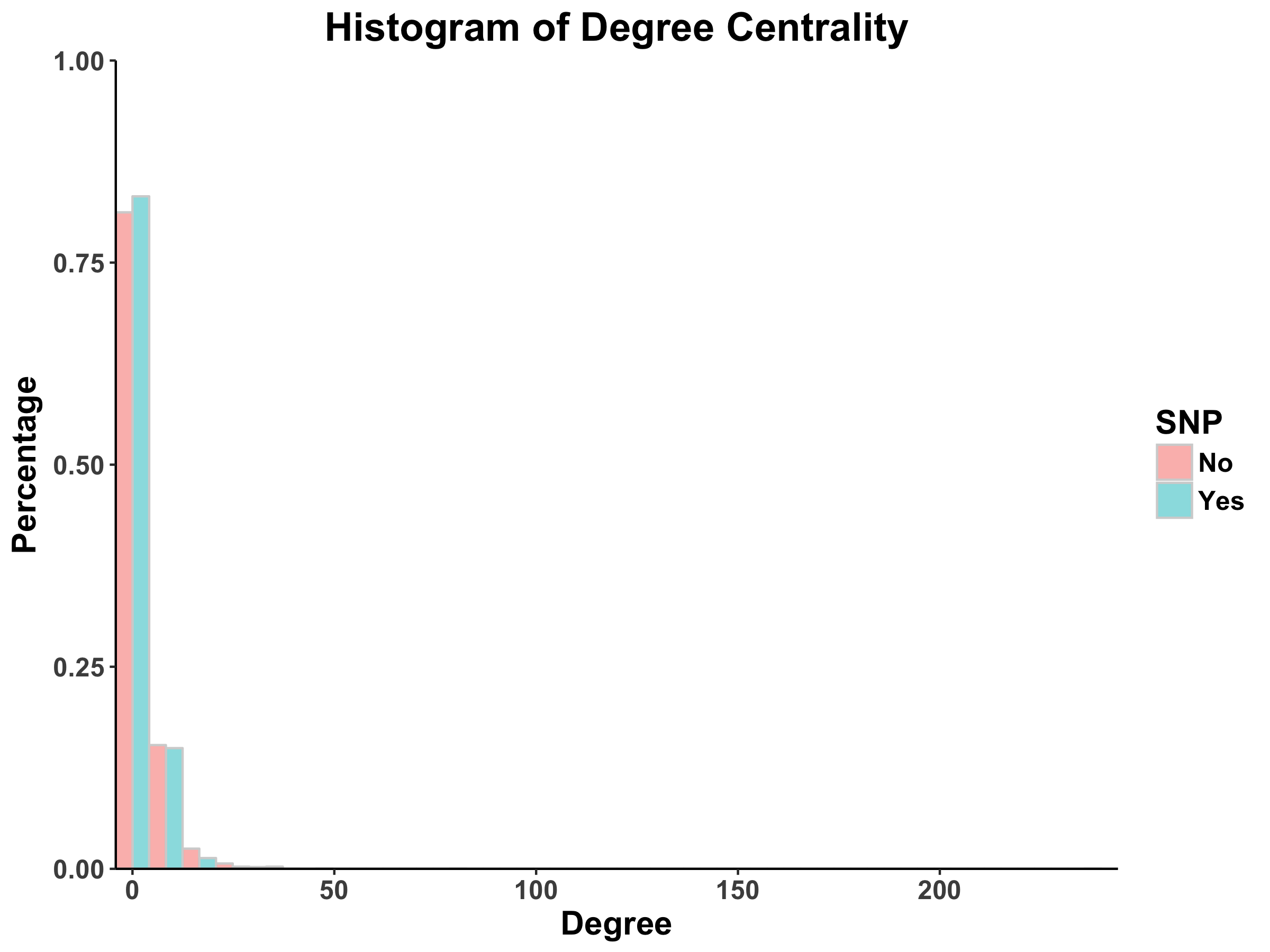
Figure 8: Betweenness Centrality Distribution in DIP Database Calculated by Cytoscape
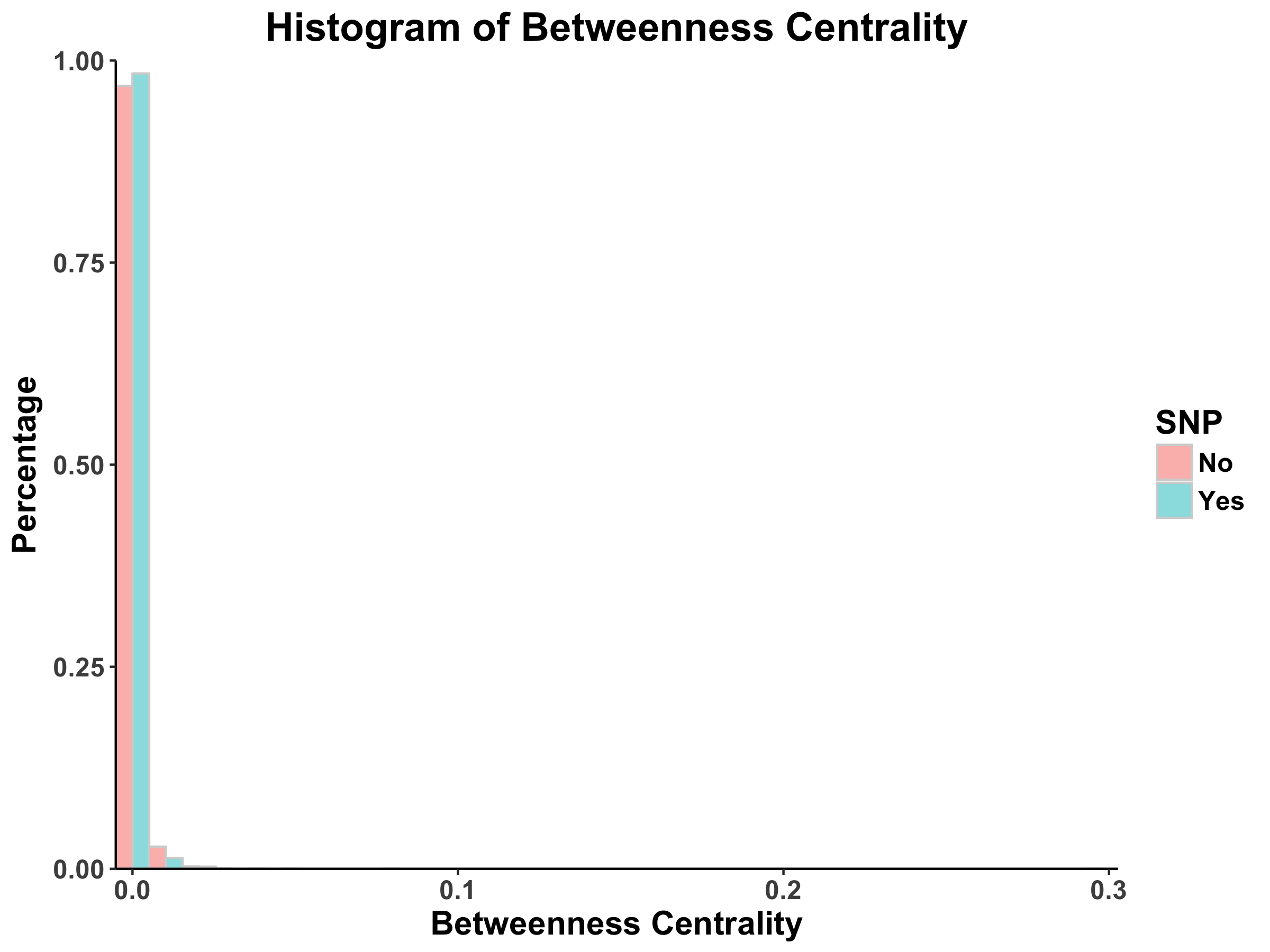
Figure 9: Degree Centrality Distribution in MINT Database Calculated by Cytoscape
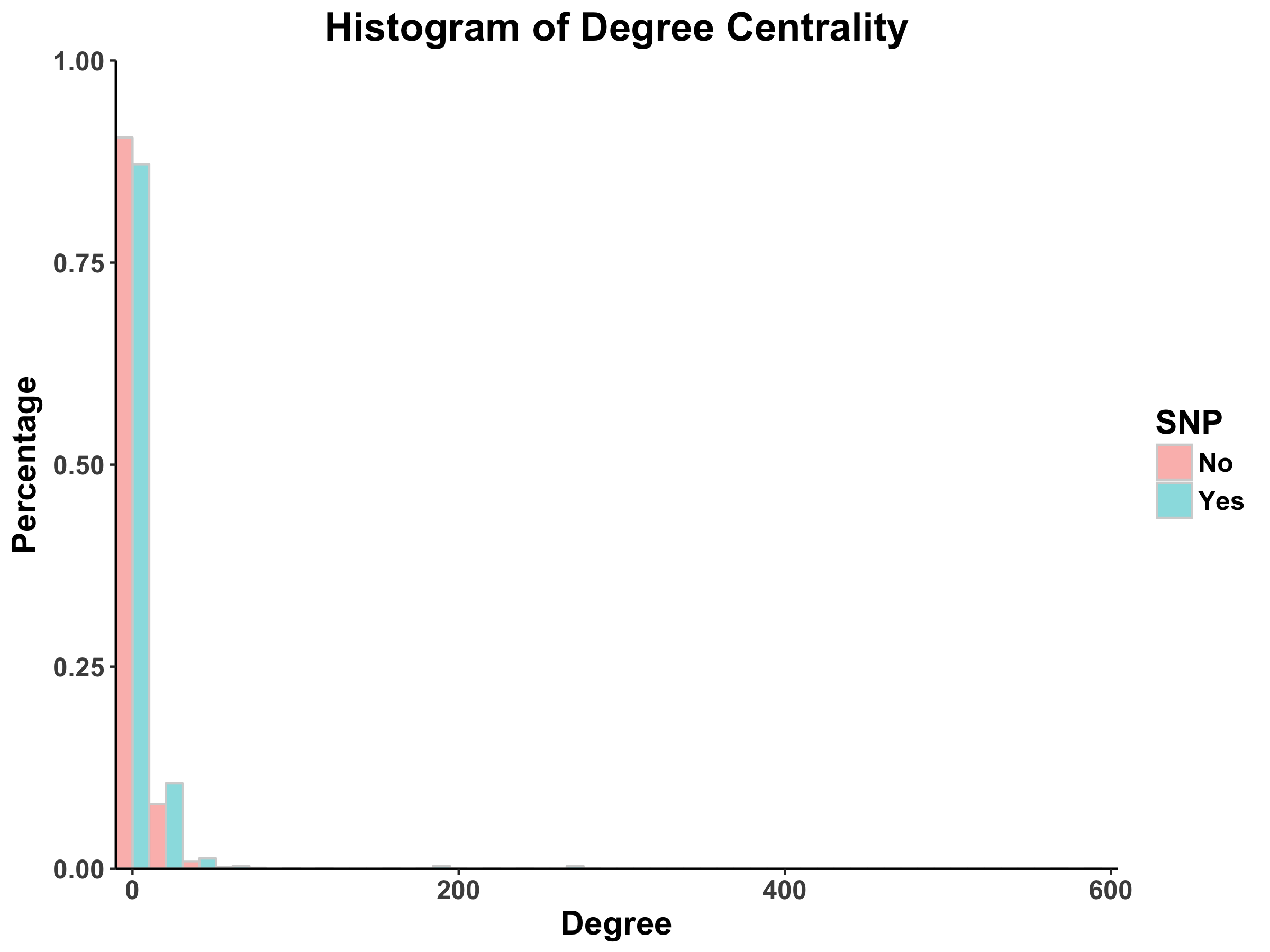
Figure 10: Betweenness Centrality Distribution in MINT Database Calculated by Cytoscape