Final project 3.1 Final Project
Part 3.1 - Network Analysis of Personal Genomes
Table of Contents
1. Introduction
For the past decade, protein networks have provided valuable insights into molecular evolution and function. New methods of measuring protein interaction have provided the data for bringing network theory and analysis to this important area. Protein networks and their properties are critical for pharmacology, disease classification, and personalized medicine. As available information grows in coverage and quality, protein networks will play an increasing role in the clinical interpretation of genetic variation. In the context of this project, protein networks allow us to better understand the importance of the Carl’s mutant coding genes and evaluate the deleteriousness of such variants.
2. Writing
2.1 Instructions
Discuss the difference of degree centrality and betweenness centrality you observed. How are these centrality measurements helpful for us to understand different mutations and the protein-protein network?
2.2 Network Theory
Application to Protein Interations: In the theory of protein-protein interaction (PPI) networks, each protein is considered to be a node. Evidence of interaction is encoded as an edge between two nodes.
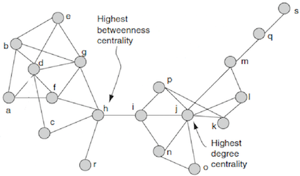
Degree Centrality: the normalized number of edges, or links, connected to a node. In the context of protein networks, this value encodes how many other proteins a certain protein is connected to. The degree centrality of a single node is its degree (number of edges) divided by (n-1), where n is the total number of nodes. Alternatively, the degree centralities can be computed as the row means (or column means) of an adjacency matrix.
Betweenness Centrality: quantifies the number of times a node acts as a bridge along the shortest path between two other nodes. Node with higher betweenness centrality have more control over the network, because more information passes through that node. In the context of protein networks, this value encodes how often a certain protein mediates the closest interaction between two unconnected proteins.
Betweenness centrality is computed as:
where $\sigma_{st}$ is the total number of shortest paths from node $s$ to node $t$, and $\sigma_{st}(v)$ is the number of those paths that pass through $v$.
Figure 1: Example of High Centrality Measures
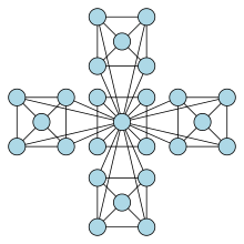
Hierarchical Network Analysis: Hierarchical models treat a network as a nested series of sub-networks. In other words, the lowest level is the original network, and every level above it collapses clusters of the network into individual nodes. These models enable the study of properties between successively larger clusters of nodes. Hierarchical models are intended for scale-free networks, which are the norm in PPI networks.
Figure 2: Example of a Simple Hierarchical Network
2.3 Databases
There exist many databases that document experimentally determined and theoretically predicted protein-protein interactions. Some commonly used PPI databases include:
- DIP: Database of Interacting Proteins
- MINT: Molecular INTeraction Database
- BIND: Biomolecular Interaction Network Database
- MIPS: Munich Information Center for Protein Sequences
- IntAct: Molecular Interaction Database
The coding and pipeline portions of this project use the DIP and MINT databases.
2.4 Observed Centrality Measures
We observed that proteins with SNPs have smaller values for both measures of centrality, meaning that they are less likely to be connected to many other nodes (degree) and less likely to help connect other nodes (betweenness. SNPs that interrupt network interactions are more likely to be deleterious and therefore less common in a healthy individual like Carl.
These centralities measurement allow us to quantitatively show the influence of an individual gene on the overall network. Genes that are connected to many nodes, or help to connect other nodes are of special interest. This is because their removal may affect a large number of other proteins and result in a more harmful mutation phenotype. We can look at which genes are affected by mutations of interest, and therefore extrapolate effects on the network at large. Thus, these measures are useful for understanding, identifying, and validating candidate mutations in the context of the whole the protein-protein network.
3. Coding
3.1 Instructions
Calculate the degree centrality and betweenness centrality of proteins containing and not containing SNPs in Carl’s genome using a PPI file.
3.2 Documentation:
We have created a script for computing the (1) degree centrality and (2) betweenness centrality of proteins in (A) proteins with Carl’s SNPs and (B) proteins without Carl’s SNPs. Data was collected from the DIP database including 4,679 proteins.
3.2.1 Usage
python3 centrality_calculation.py -i <input file> -a <annotation file> -n <dip ppi file>
3.2.2 Example
python3 centrality_calculation.py -i input.txt -a map_table.txt -n dip.txt
3.2.3 Input File
Z.3DStruct_annotation.txt
3.2.4 Annotation File
From uniprot id to gene name:
From To
P62161 Calm1
3.2.5 DIP PPI file
DIP PPI file can be downloaded online. We provide a DIP PPI file in the package.
3.3 Results:
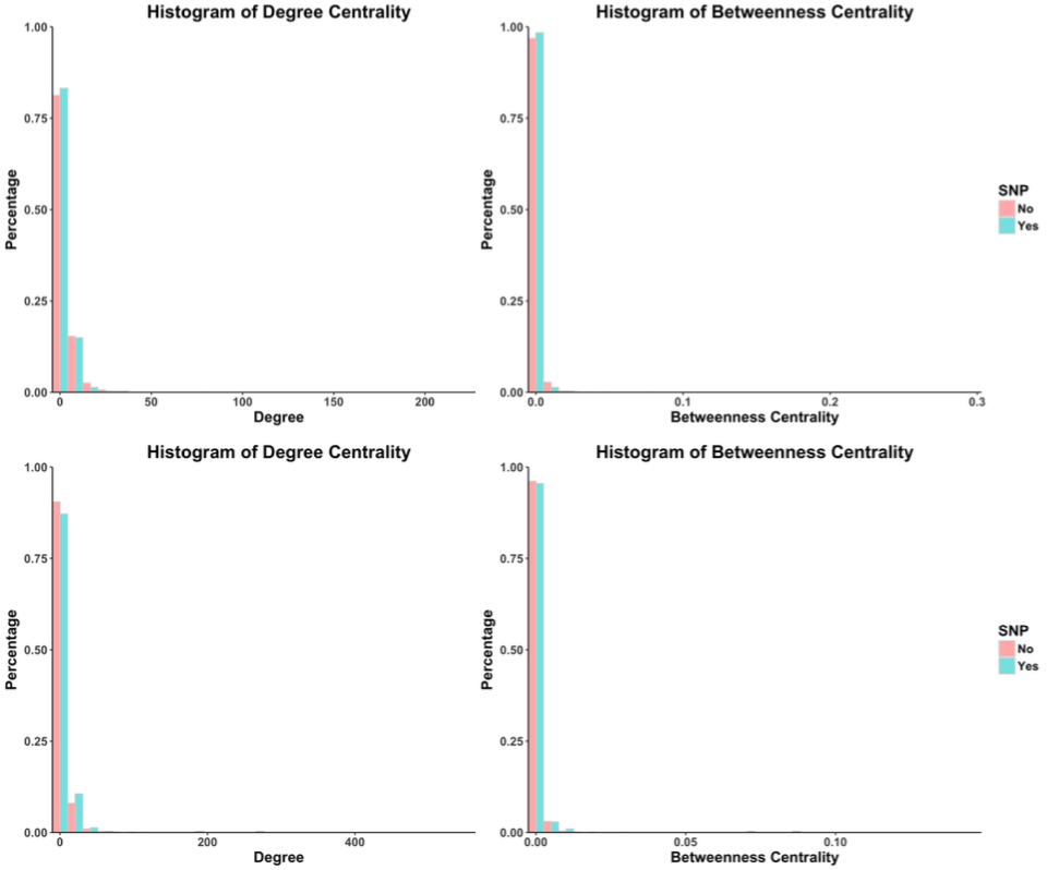
Figure 3: Network properties of proteins with and without Carl’s SNPs
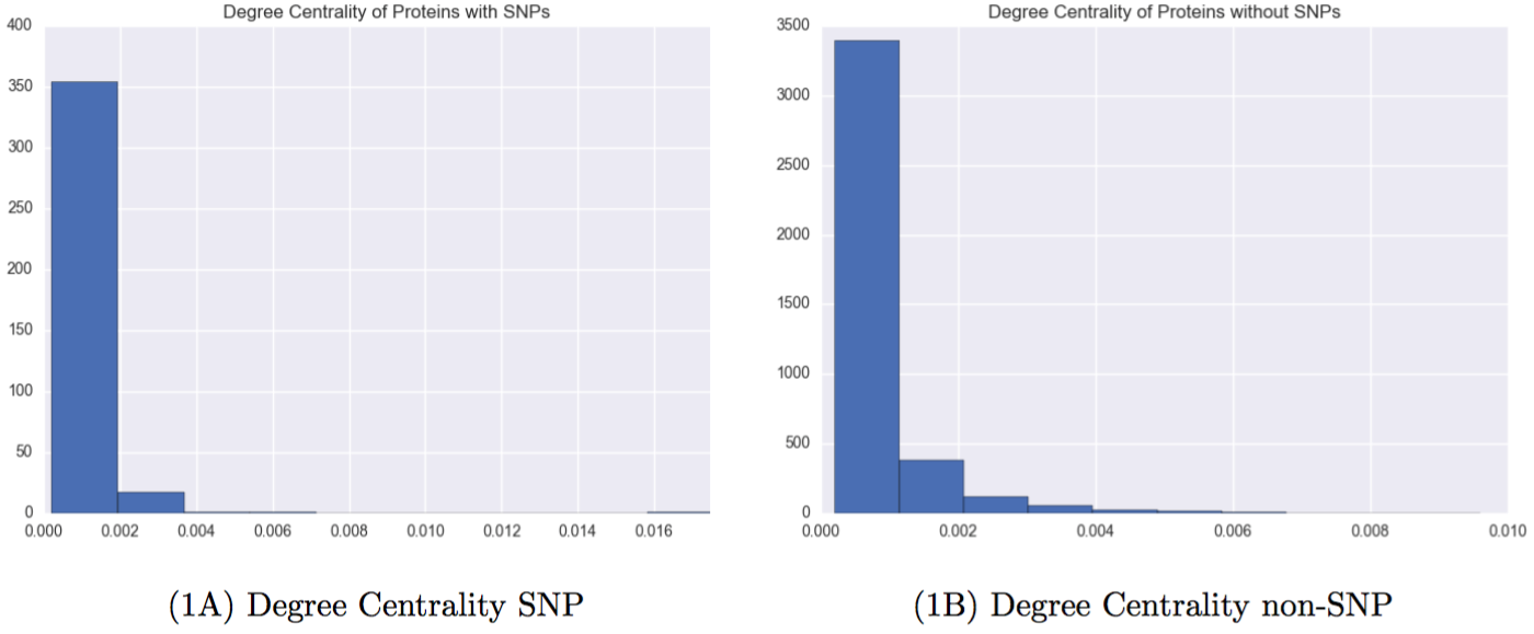
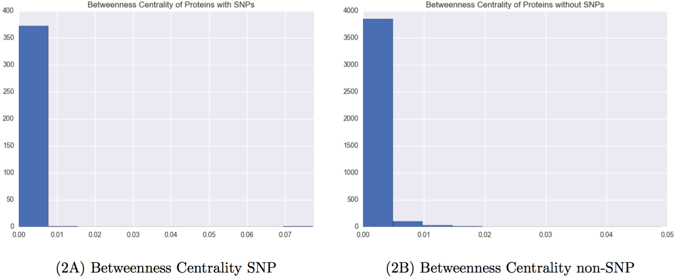
It is clear that proteins with SNPs are shifted left on both measures of centrality, meaning that they are both less likely to be connected to many other nodes, and less likely to help connect other nodes.
4. Pipeline
4.1 Instructions
Use Cytoscape or other softwares to visualize the protein-protein network. Check the centrality calculations with the software and demonstrate one or two examples. Perform hierarchical network analysis and determine if there is enriched or depleted mutation in each hierarchy.
4.2 Documentation:
We have chosen to use Cytoscape to visualize the protein-protein network. In each plot, the genes with Carl’s SNPs are marked in red, and the genes without SNPs are marked in green. The node size is proportional to its degree.
The gene name mapping is based on ENSEMBL transcript ID - uniprotKB ID pairs. The number of genes recorded in Carl’s coding region SNPs file in DIP is 375 and the number in MINT is 306. All the analyses are done by Cytoscape. Histograms are plotted in R ggplot2.
Lastly, hierarchical network analysis was performed to look for enrichment or depletion of mutations in different hierarchies. Although the interactomes DIP and MINT do not have regulatory relationship recorded, it might still be useful to check the hierarchy in network structure like directed graphs. The goal is to separate the graph in a hierarchy. However, I did not find any available tools to use or algorithms to implement on undirected graphs for hierarchical analysis. Note that, HirNet by Cheng C et al. is designed for directed network, but here we use it to catch a glimpse of the network structure. It does not necessarily reflect any regulatory features for the network itself. Fisher’s exact test was used to test for enrichment of SNPs in each hierarchical layer.
4.3 Results:
4.3.1 Visualizing the Protein-Protein Network
Figure 4: Visualized Network from DIP
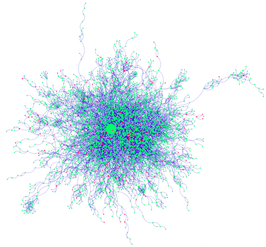
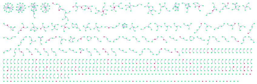
Figure 5: Visualized Network from MINT
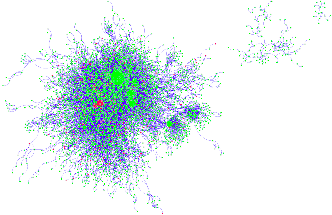
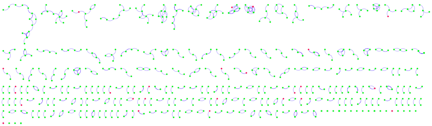
Because of the large number of nodes, it is not immediately obvious whether the red genes (with SNPs) are enriched at the borders and in smaller nodes, as would be expected. However, by inspecting the details below each map, such a pattern may be deduced.
4.3.2 Checking Centrality Calculations with Cytoscape
Cytoscape was used to replicate the histograms for degree centrality and betweenness centrality. This time, paired barplots are used for easy comparison.
Figure 6: Replicated network properties of genes with and without Carl’s SNPs
4.3.3 Hierarchical Network Analysis
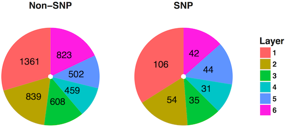
The DIP and MINT network are cut into 6 layers. Fisher’s exact is used to test the enrichment of genes with SNP in Carl’s genome for different layers. The distribution of genes in the 6 layers is shown as below.
Figure 7: Distribution of genes across layers in DIP
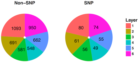
Figure 8: Distribution of genes across layers in MINT
4.3.4 Detection of Mutation Enrichment or Depletion in Each Hierarchical Layer
Based on the result of Fisher’s exact test ($\alpha$ = 0.05), there is no significant enrichment in any layers for these network, which may indicate genes with SNP are not clustered or scattered in specific patterns compared to those without SNPs.
Table 1: P-values for Mutation Enrichment in 6 Hierarchical Layers
| Hierarchy | DIP p-value | MINT p-value |
|---|---|---|
| 1 | 0.90 | 0.06 |
| 2 | 0.33 | 0.69 |
| 3 | 0.14 | 0.87 |
| 4 | 0.32 | 0.54 |
| 5 | 0.52 | 0.05 |
| 6 | 0.74 | 0.98 |
5. Conclusions
A network analysis of Carl’s personal genome reveals some properties of his genes with SNPs. By two separate metrics, these genes have been quantitatively shown to have lower influence on the overall protein network. The Cytoscape visualization further helps demonstrate this pattern. These network plots also reveal a few genes (the large, red nodes) that are more likely to be problematic based on their positioning (between other nodes) and degree (large number of direct connections). None of these findings can definitely demonstrate pathogenicity. Still, these metrics are valuable for identifying and validating candidate mutations to report. Hierarchical analysis was employed to model the protein network, but there did not appear to be significant SNP enrichment in any of the 6 resultant layers.
Source code
6. References
- Barabási A-L, Oltvai ZN. Network biology: understanding the cell’s functional organization. Nat Rev Genet. 2004;5(2):101-113. doi:10.1038/nrg1272.
- Ideker T, Sharan R. Protein networks in disease. Genome Res. 2008;18(4):644-652. doi:10.1101/gr.071852.107.
- Shannon P, Markiel A, Ozier O, et al. Cytoscape: A software Environment for integrated models of biomolecular interaction networks. Genome Res. 2003;13(11):2498-2504. doi:10.1101/gr.1239303.